오늘은 '위스콘신 대학의 유방암 진단 분류 데이터'를 가지고 데이터 전처리를 진행해 볼 것이다.
원래 문제없는 데이터인데, 실습을 위해서 여기저기 결측치 값을 일부러 만들었다.
정형 데이터에 대해서 결측치 처리하는 방법과 범주형 데이터의 정규화 등 데이터를 전처리하는 과정에 대해서 알아보자.
전반적인 데이터 전처리 과정은 아래와 같다.
1. 데이터 불러오기
2. Explorating
3. 결측치 처리: strategy(remove, imputation)
4. Scaling
5. Data Split
0. 라이브러리 불러오기
import numpy as np
import pandas as pd
import matplotlib.pyplot as plt
import sklearn
import seaborn as sns
1. 데이터 불러오기
wbsc = pd.read_csv('./wbcs_data_modified.csv')
wbsc
# 통계 알아보기(평균, 중앙값, 최빈값 등)
wbsc.describe()

# columns에 대한 정보 한눈에 보기
wbsc.info()
2. 결측치 처리
1) 결측치 데이터 알아보기
# 결측치 값이 있을 경우 True, 데이터가 있는 경우 False
wbsc.isnull()

# 각 column의 결측치 개수
wbsc.isnull().sum()
이 데이터에서는 radius_mean(49개), concavity_se(18개), area_worst(18개)에 결측치가 있다고 나온다.
결측치값을 그래프로 보기 위해서는 missingno 라이브러리를 가져와야 한다.
!pip install missingno
import missingno as msno- Matrix: 결측치 분포 확인
msno.matrix(wbsc)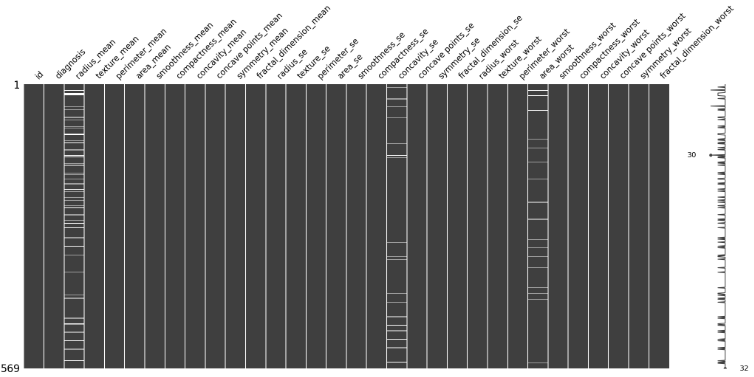
- Bar: 결측치 개수 확인
msno.bar(wbsc)
2) 대체 또는 제거
우선, 원본 파일을 새로운 곳에 복사를 해준다.
df = wbsc   # shallow copy
df- 결측치 삭제
msno.matrix(df.dropna())
df_remove = df.dropna()   # 삭제한 데이터 복사
- 결측치 대체: 평균 or 최빈값
from sklearn.impute import SimpleImputer

df2 = wbsc

imputer_mean = SimpleImputer(strategy="mean")   # 평균값으로 결측치를 대체하는 클래스 인스턴스
imputer_mf = SimpleImputer(strategy="most_frequent")   # 최빈값으로 결측치를 대체하는 클래스 인스턴스
둘 중 필요한 것을 선택해서 사용하면 된다. 어떤 걸 선택하는지에 따라 모델의 성능이 달라질 수 있다.
# 평균값 대체
df2 = wbsc

df2['radius_mean'] = imputer_mean.fit_transform(df2[['radius_mean']])
df2['concavity_se'] = imputer_mean.fit_transform(df2[['concavity_se']])
df2['area_worst'] = imputer_mean.fit_transform(df2[['area_worst']])

# 최빈값 대체
df3 = wbsc

df3['radius_mean'] = imputer_mf.fit_transform(df3[['radius_mean']])
df3['concavity_se'] = imputer_mf.fit_transform(df3[['concavity_se']])
df3['area_worst'] = imputer_mf.fit_transform(df3[['area_worst']])
3) 확인하기
# 데이터 개수 확인
df_remove.shape, df2.shape, df3.shape

# 데이터 통계 확인
df.describe(), df_remove.describe(), df2.describe(), df3.describe()
3. 범주형 데이터 Encoding
df['diagnosis'].unique()
encode_diag이라는 새로운 column을 만들어, M이라면 1, B라면 0의 숫자형 데이터로 변환해 준다.
# one-hot encoding
def one_hot(row):
    if 'M' in row: return 1
    else: return 0

# apply()
df['encode_diag'] = df['diagnosis'].apply(one_hot)  # 새로운 column이 생김
df.tail(20)
아까 전처리했던 데이터에도 적용해주자.
df2['encode_diag'] = df2['diagnosis'].apply(one_hot)
df3['encode_diag'] = df3['diagnosis'].apply(one_hot)

df2[["diagnosis", "encode_diag"]]
※ 데이터 Scatter Plot
num_columns = 3
num_rows = (df.shape[1] + num_columns - 1) // num_columns
fig, axes = plt.subplots(num_rows, num_columns, figsize=(25, 100))

for i, column in enumerate(df.columns):
    ax = axes[i // num_columns, i % num_columns]
    ax.scatter(df.index, df[column], label=column)
    ax.set_xlabel('Index')
    ax.set_ylabel('Values')
    ax.set_title(f'Scatter Plot - {column}')
    ax.legend()
4. 데이터 정규화 (Data Normalization)
# MinMax Normalization
from sklearn.preprocessing import MinMaxScaler as MMS
# Dataset -> split; X: imput, y: label
# x: Label을 제외한 모든 column
# y: Label <- diagnosis => encode_diag
x = df.drop(['id', 'diagnosis', 'encode_diag'], axis=1) # axis = 1: column drop
y = df['encode_diag']
df.shape, x.shape, y.shapescaler = MMS()
scaler.fit(x)
x_norm = scaler.transform(x)
x_norm = pd.DataFrame(x_norm, columns=x.columns)
# x_norm = pd.DataFrame(scaler.fit_transform(x), columns=x.columns)
x_norm
5. Data Split
# Train:Test = 7:3
from sklearn.model_selection import train_test_split as tts
x_train, x_test, y_train, y_test = tts(x_norm, y, test_size=0.3, random_state=812)
x_train.shape, x_test.shape, y_train.shape, y_test.shape그리고 전저리된 데이터에도 적용을 시키자.
x2 = df_remove.drop(['id', 'diagnosis', 'encode_diag'], axis=1)
y2 = df_remove['encode_diag']
※ 해당 카테고리는 딥노이드, 오픈놀, 앙트비에서 주최하는 '<스타트업 유니버시티: DX Challenge 교육> AI+X 역량 강화 트랙'에 대한 기록입니다.
'[AI+X 역량 강화] 인공지능 > 2) 주특기 심화: 머신러닝, 딥러닝' 카테고리의 다른 글
| 딥러닝 활용 프로젝트 // 나이 예측앱, 백혈병 분류앱 만들기 (0) | 2023.09.20 |
|---|---|
| [머신러닝] #2 머신러닝을 위한 데이터 전처리 // 특성공학, 결측값, 범주형 변수 처리 (0) | 2023.09.09 |
| DX AI 산업 특강 // 챗GPT로 웹페이지 만들기 (0) | 2023.09.07 |
| [머신러닝]#1 머신러닝의 이해 // 데이터 종류, 스팸 필터, 머신러닝 특징 (0) | 2023.09.05 |


